Hoek-Brown criterion

Calculates the Hoek-Brown criterion for the given data and for the given level of stress (unit weight and depth), and an option for plotting it.

Usage

Hoek_Brown(
  sig.ci,
  GSI,
  mi,
  MR,
  D,
  height,
  unit.weight,
  use = c("general", "tunnels", "slopes")
)

Hoek_Brown_plot(HB)

Arguments

sig.ci: The unconfined compressive strength of the intact rock, in MPa
GSI: The Geological Strength Index
mi: The intact rock constant
MR: the modulus ratio
D: The quality of the explosive campaing design
height: The height or depth for which to determine the stress level and parameters
unit.weight: The unit weight of the rock, in kN/m3
use: The use expected for the rock mass (general, tunnels, or slopes)
HB: The result from running Hoek_Brown()

Value

For Hoek_Brown(): a list with a list of the resulting parameters of the rock mass and 3 data frames: Shear envelopes for Mohr-Coulomb and Hoek-Brown criteria, Principal stresses envelopes for Mohr-Coulomb and Hoek-Brown criteria, and stress level for the given height and unit weight

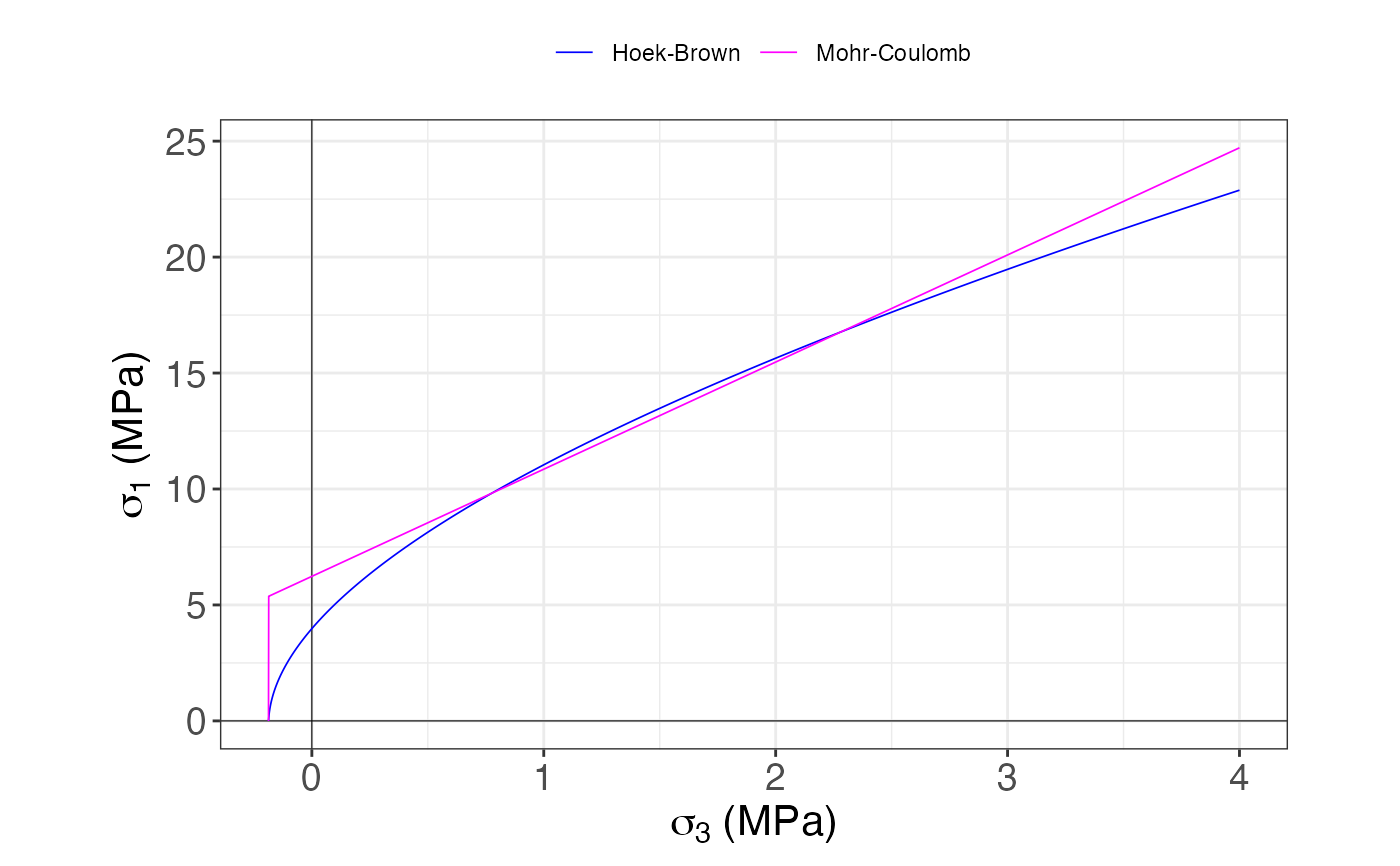
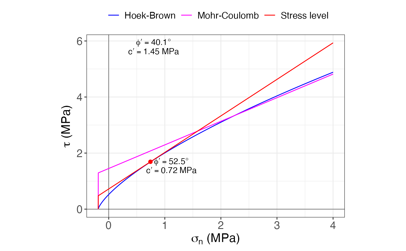
For Hoek_Brown_plot(): a list with two ggplot objects for the Hoek-Brown criterion (principal stresses and normal-shear stresses)

Details

Tables for some of the input parameters can be found in the directory where the package is installed, just run the following command to find this path: system.file(package = "GMisc")

References

Hoek, E. & Brown, E. T. (1980). Empirical strength criterion for rock masses. J. Geotech. Eng. Div. ASCE 106 (GT9): 1013-1035.

Hoek, E., Carranza-Torres, C. & Corkum, B. (2002). Hoek-Brown Failure Criterion - 2002 Edition. Proc. NARMS-TAC Conference, Toronto. 267-273.

Hoek, E. & Marinos, P. (2007). A brief history of the development of the Hoek-Brown criterion. Soils and Rocks, No. 2.

Examples

sig.ci = 16
GSI = 75
mi = 13
MR = 300
D = 0
height = 40
unit.weight = 18.6
HB = Hoek_Brown(sig.ci, GSI, mi, MR, D, height, unit.weight)
HB
#> $Results
#> $Results$sig.ci
#> [1] 16
#> 
#> $Results$GSI
#> [1] 75
#> 
#> $Results$mi
#> [1] 13
#> 
#> $Results$D
#> [1] 0
#> 
#> $Results$mb
#> [1] 5.32
#> 
#> $Results$s
#> [1] 0.0622
#> 
#> $Results$a
#> [1] 0.501
#> 
#> $Results$MR
#> [1] 300
#> 
#> $Results$Ei
#> [1] 4800
#> 
#> $Results$sig.3.max
#> [1] 4
#> 
#> $Results$sig.t
#> [1] -0.187
#> 
#> $Results$sig.c
#> [1] 3.98
#> 
#> $Results$sig.cm
#> [1] 5.87
#> 
#> $Results$Erm
#> [1] 3918.48
#> 
#> $Results$phi
#> [1] 40.1
#> 
#> $Results$c
#> [1] 1.45
#> 
#> $Results$phi.h
#> [1] 52.5
#> 
#> $Results$c.h
#> [1] 0.72
#> 
#> 
#> $shear
#> # A tibble: 12,564 × 3
#>     sig.n crit           tau
#>     <dbl> <chr>        <dbl>
#>  1 -0.187 Hoek-Brown   0.001
#>  2 -0.187 Mohr-Coulomb 0    
#>  3 -0.187 Stress level 0    
#>  4 -0.186 Hoek-Brown   0.011
#>  5 -0.186 Mohr-Coulomb 1.29 
#>  6 -0.186 Stress level 0.478
#>  7 -0.185 Hoek-Brown   0.018
#>  8 -0.185 Mohr-Coulomb 1.29 
#>  9 -0.185 Stress level 0.479
#> 10 -0.184 Hoek-Brown   0.024
#> # ℹ 12,554 more rows
#> 
#> $princ.stress
#> # A tibble: 8,376 × 3
#>     sig.3 crit         sig.1
#>     <dbl> <chr>        <dbl>
#>  1 -0.187 Hoek-Brown   0    
#>  2 -0.187 Mohr-Coulomb 0    
#>  3 -0.186 Hoek-Brown   0.113
#>  4 -0.186 Mohr-Coulomb 5.37 
#>  5 -0.185 Hoek-Brown   0.231
#>  6 -0.185 Mohr-Coulomb 5.38 
#>  7 -0.184 Hoek-Brown   0.323
#>  8 -0.184 Mohr-Coulomb 5.38 
#>  9 -0.183 Hoek-Brown   0.402
#> 10 -0.183 Mohr-Coulomb 5.39 
#> # ℹ 8,366 more rows
#> 
#> $stress.level
#> # A tibble: 1 × 3
#>    sign   tau crit        
#>   <dbl> <dbl> <chr>       
#> 1 0.744  1.69 Stress level
#> 
Hoek_Brown_plot(HB)
#> $princ.stresses

#> 
#> $normal.shear

#>