Test for common axis direction (axial)

Tests whether two or more groups of 3-D orientations share a common principal or polar axis. The dominant fabric type—cluster (point) or girdle—is determined from the pooled PGR indices: if the point index dominates the principal eigenvector (V1) is tested; if the girdle index dominates the polar eigenvector (V3) is tested. When the pooled data are essentially random no formal test is performed. If the null hypothesis is not rejected the pooled axis and its confidence cone are overlaid in the stereonet. Per-group axes and their confidence cones are always shown in distinct colours.

Usage

dir_aov_spher_ax(
  trd,
  plg,
  grp,
  data = NULL,
  conf.level = 0.95,
  type = c("line", "dir", "strike")
)

Arguments

trd

Numeric vector of trend values in degrees, or an unquoted column name when data is supplied. For lines: trend of the lineation. For planes: dip direction or strike depending on type.

plg

Numeric vector of plunge values in degrees, or an unquoted column name when data is supplied. For lines: plunge. For planes: dip angle.

grp

A vector (factor or character) of group labels, or an unquoted column name when data is supplied. Must be the same length as trd and plg.

data

A data frame (or tibble) containing the columns referenced by trd, plg, and grp. Default NULL (use vectors directly).

conf.level

Numeric. Confidence level for per-group and pooled axis confidence cones. Default 0.95.

type

Character. How to interpret the input orientations:

"line"

(default) Trend and plunge of a lineation.

"dir"

Dip direction and dip angle of a plane (pole used internally).

"strike"

Strike (right-hand rule) and dip angle of a plane (pole used internally).

Value

A named list whose components depend on the pooled fabric type:

PGR

Tibble of pooled fabric indices: P (point), G (girdle), R (random), B (= 1 − R).

statement

Character string summarising the test conclusion. One of: "Samples come from a distribution with common principal/polar axis", "Principal/Polar axis differs between samples", or "Pooled data follows a random distribution" (when R dominates).

axial_g

Tibble with per-group axis statistics: group label grp, sample size n, trend trd, plunge plg, confidence cone half-width cone (degrees), concentration parameter kappa, eigenvalue lambda, and normalised eigenvalue S. Present only when the data are not random.

axial_res

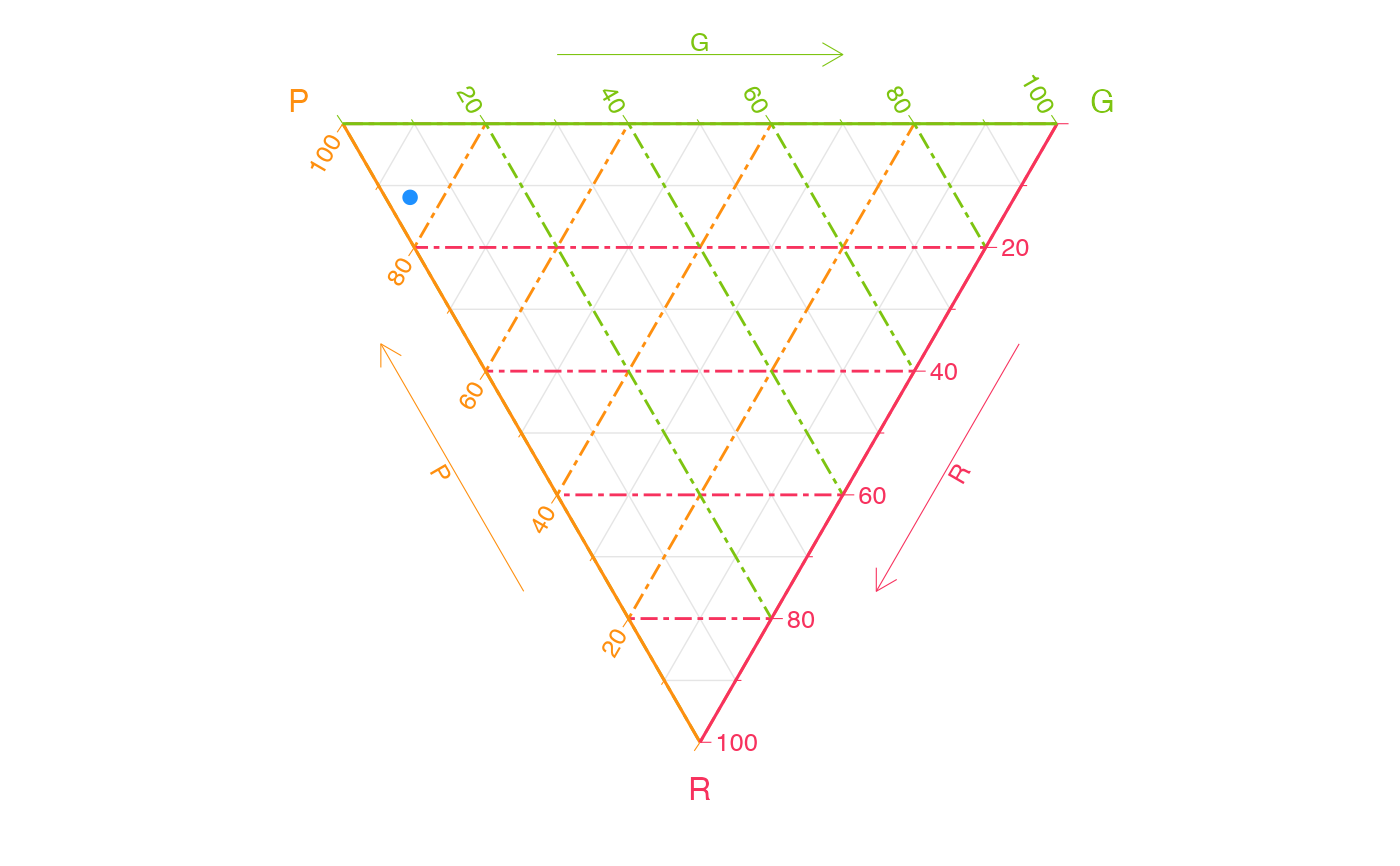
Tibble with the test statistic Nr, degrees of freedom df, and p-value p.value. When the null hypothesis is not rejected, also includes the pooled axis trend trd, plunge plg, confidence cone cone, kappa, sample size N, lambda, and S. Present only when the data are not random.

pgrplot

A ggtern Point–Girdle–Random ternary diagram. Present only when the null hypothesis is not rejected.

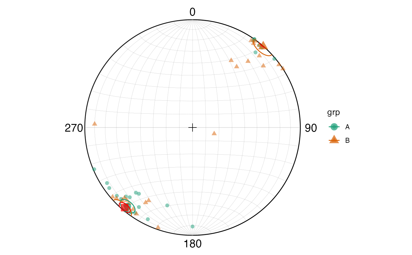
stereoplot

A ggplot equal-area stereonet showing data points per group, per-group axes (coloured squares) with confidence cones, and—when the null is not rejected—the pooled axis with its confidence cone (red for principal, blue for polar axis).

References

Fisher, N. I., Lewis, T., & Embleton, B. J. J. (1987). Statistical analysis of spherical data. Cambridge University Press.

See also

Other directional statistics: dir_aov_spher_vec(), dir_stats_circ(), dir_stats_spher(), rose_diag_circ(), rose_diag_spher()

Examples

# From a data frame
csv_path <- system.file("spherical_data_ax_bp_aov.csv", package = "GMisc")
df <- utils::read.csv(csv_path)
dir_aov_spher_ax(trend, plunge, type, data = df)
#> $PGR
#> # A tibble: 1 × 4
#>       P      G     R     B
#>   <dbl>  <dbl> <dbl> <dbl>
#> 1 0.846 0.0346 0.119 0.881
#> 
#> $statement
#> [1] "Samples come from a distribution with common principal axis"
#> 
#> $axial_g
#> # A tibble: 2 × 8
#>   grp       n   trd   plg  cone kappa lambda     S
#>   <chr> <int> <dbl> <dbl> <dbl> <dbl>  <dbl> <dbl>
#> 1 A        25 220.   5.79  4.93 16.9    23.5 0.939
#> 2 B        25  41.1  0.3   6.34  8.59   21.8 0.873
#> 
#> $axial_res
#> # A tibble: 1 × 12
#>   sigma      g    Nr    df p.value   trd   plg  cone kappa     N lambda     S
#>   <dbl>  <dbl> <dbl> <dbl>   <dbl> <dbl> <dbl> <dbl> <dbl> <int>  <dbl> <dbl>
#> 1 0.847 0.0664  1.92     2   0.384  220.  2.97  3.62  11.0    50   45.2 0.903
#> 
#> $pgrplot

#> 
#> $stereoplot

#>