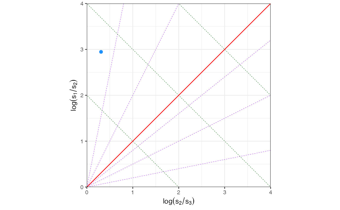
Spherical (3-D directional) descriptive statistics

Computes descriptive statistics for a sample of 3-D orientations (lines or planes) using spherical statistics. The function calculates the mean resultant vector, concentration parameter, and confidence cone for the mean direction, performs an eigenvalue / eigenvector decomposition of the orientation matrix, estimates distribution parameters for Watson bipolar, Watson girdle, and Bingham distributions, and returns several diagnostic plots (stereonet, eigenvalue ratio plot, and PGR ternary diagram).

Usage

dir_stats_spher(
  trd,
  plg,
  data = NULL,
  conf.level = 0.95,
  type = c("line", "dir", "strike"),
  plot = c("all", "eig", "mean")
)

Arguments

trd

Numeric vector of trend values in degrees, or an unquoted column name when data is supplied. For lines: trend of the lineation. For planes: dip direction or strike depending on type.

plg

Numeric vector of plunge values in degrees, or an unquoted column name when data is supplied. For lines: plunge of the lineation. For planes: dip angle.

data

A data frame (or tibble) containing the columns referenced by trd and plg. Default NULL (use vectors directly).

conf.level

Numeric. Confidence level for mean-direction and eigenvector confidence cones/ellipses. Default 0.95.

type

Character. How to interpret the input orientations:

"line": (default) Trend and plunge of a lineation.
"dir": Dip direction and dip angle of a plane (converted internally to the pole).
"strike": Strike (right-hand rule) and dip angle of a plane (converted internally to the pole).

plot

Character. Which stereonet to include in the output:

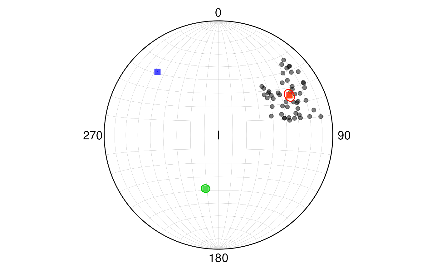
"all": (default) Data points, mean vector with confidence cone (gold), and all three eigenvectors with their confidence cones (red, green, blue).
"eig": Data points and eigenvectors with confidence cones only.
"mean": Data points and mean vector with confidence cone only.

Value

A named list with the following components:

eigen_values: 1 × 3 matrix of normalised eigenvalues \(S_1 \ge S_2 \ge S_3\) of the orientation matrix.
eigen_vectors: 3 × 3 data frame of eigenvectors (direction cosines), columns V1–V3.
orientation_matrix: 3 × 3 orientation (scatter) matrix.
trend_plunge: 2 × 3 matrix with trend (row 1) and plunge (row 2) of each eigenvector in degrees.
dir_dip: 2 × 3 matrix with dip direction (row 1) and dip (row 2) of each eigenvector in degrees.
vector_stats: Tibble with mean direction statistics: trd, plg, strike, dir, dip, resultant length R, mean resultant length Rbar, concentration parameter kappa, confidence cone half-width cone (degrees), and sample size N.
axis_stats_watson: Tibble with confidence cone half-widths for each eigenvector (V1_cone, V2_cone, V3_cone) and estimated concentration parameters for the Watson bipolar (kappa_bipolar) and Watson girdle (kappa_girdle) distributions.
axis_stats_aniso: Data frame (3 × 3) with Bingham κ values and Watson confidence ellipse semi-axes (degrees) for each eigenvector.
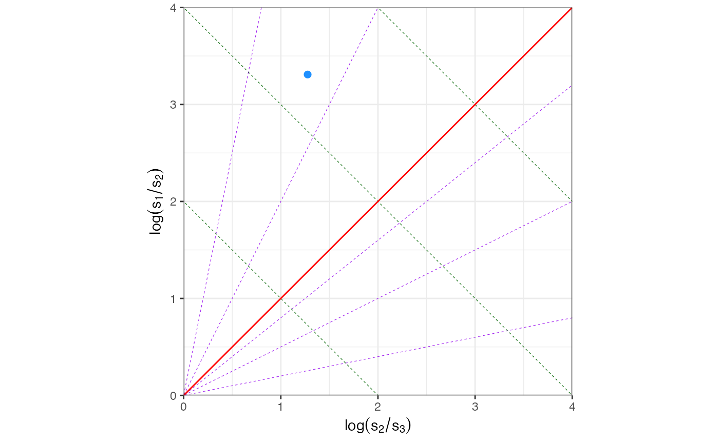
PointGirdleRandom: Tibble of fabric indices: P (point/cluster), G (girdle), R (random), B (= 1 − R), eigenvalue ratios \(S_1/S_2\), \(S_1/S_3\), \(S_2/S_3\), log-ratios r1 and r2, Woodcock's shape K and strength C parameters, intensity index I, and distance index D.
eigenplot: A ggplot object: log-ratio eigenvalue plot (\(\ln(S_2/S_3)\) vs \(\ln(S_1/S_2)\)) with K-lines and C-isolines.
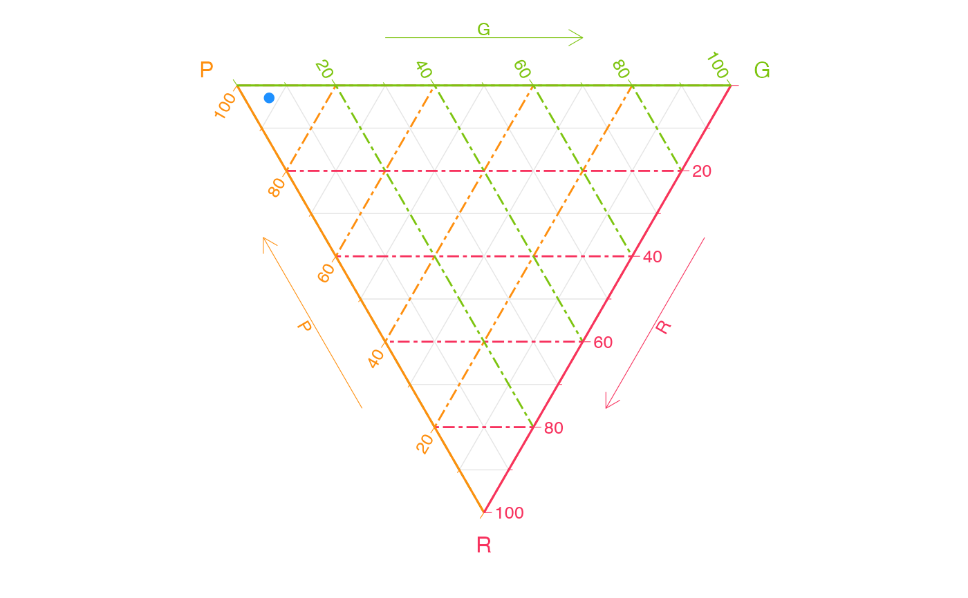
pgrplot: A ggtern object: Point–Girdle–Random ternary diagram.
stereoplot: A ggplot equal-area stereonet according to the plot argument.

References

Fisher, N. I., Lewis, T., & Embleton, B. J. J. (1987). Statistical analysis of spherical data. Cambridge University Press.

Mardia, K. V., & Jupp, P. E. (2000). Directional Statistics. John Wiley & Sons.

Woodcock, N. H. (1977). Specification of fabric shapes using an eigenvalue method. Geological Society of America Bulletin, 88(9), 1231–1236. https://doi.org/10.1130/0016-7606(1977)88%253C1231:SOFSUA%253E2.0.CO;2

Vollmer, F. W. (1990). An application of eigenvalue methods to structural domain analysis. Geological Society of America Bulletin, 102(6), 786–791. https://doi.org/10.1130/0016-7606(1990)102%253C0786:AAOEMT%253E2.3.CO;2

Lisle, R. J. (1985). The use of the orientation tensor for the description and statistical testing of fabrics. Journal of Structural Geology, 7(1), 115–117. https://doi.org/10.1016/0191-8141(85)90119-1

Examples

# Lines supplied as plain vectors
set.seed(123)
trds <- runif(50, 40, 80)
plgs <- runif(50, 10, 50)
res <- dir_stats_spher(trds, plgs)
res$vector_stats
#> # A tibble: 1 × 13
#>     trd   plg strike   dir   dip     R  Rbar kappa  cone     N     x     y     z
#>   <dbl> <dbl>  <dbl> <dbl> <dbl> <dbl> <dbl> <dbl> <dbl> <int> <dbl> <dbl> <dbl>
#> 1  60.7  29.6   151.  241.  60.4  48.3 0.966  29.1  3.80    50 0.425 0.759 0.494
res$stereoplot


# Planes given as dip direction / dip, eigenvectors only on stereonet
dir_stats_spher(trds, plgs, type = "dir", plot = "eig")
#> $eigen_values
#>             V1     V2     V3
#> lambda 47.7667 1.7460 0.4873
#> S       0.9553 0.0349 0.0097
#> 
#> $eigen_vectors
#>           V1        V2            V3
#> x -0.2301643 0.4246250 -0.8756243305
#> y -0.4190570 0.7688369  0.4829917857
#> z  0.8783027 0.4781040  0.0009832548
#> 
#> $orientation_matrix
#>           [,1]       [,2]       [,3]
#> [1,]  3.218914   4.971111  -9.302181
#> [2,]  4.971111   9.534007 -16.938923
#> [3,] -9.302181 -16.938923  37.247079
#> 
#> $trend_plunge
#>         V1    V2     V3
#> trd 241.22 61.09 151.12
#> plg  61.44 28.56   0.06
#> 
#> $dir_dip
#>        V1     V2     V3
#> dir 61.22 241.09 331.12
#> dip 28.56  61.44  89.94
#> 
#> $vector_stats
#> # A tibble: 1 × 13
#>     trd   plg strike   dir   dip     R  Rbar kappa  cone     N      x      y
#>   <dbl> <dbl>  <dbl> <dbl> <dbl> <dbl> <dbl> <dbl> <dbl> <int>  <dbl>  <dbl>
#> 1  241.  61.4   331.  61.2  28.6  48.9 0.977  43.1  3.10    50 -0.231 -0.419
#> # ℹ 1 more variable: z <dbl>
#> 
#> $axis_stats_watson
#> # A tibble: 1 × 5
#>   V1_cone V2_cone V3_cone kappa_bipolar kappa_girdle
#>     <dbl>   <dbl>   <dbl>         <dbl>        <dbl>
#> 1    3.11    2.76    71.7          22.9        -51.3
#> 
#> $axis_stats_aniso
#>                       V1      V2      V3
#> bingham kappa      0.000 -16.255 -51.302
#> watson max ellipse 3.883  14.936  14.951
#> watson min ellipse 2.010   3.778   1.679
#> 
#> $PointGirdleRandom
#> # A tibble: 1 × 13
#>       P      G      R     B     I     D     K     C s1.s2 s1.s3 s2.s3    r1
#>   <dbl>  <dbl>  <dbl> <dbl> <dbl> <dbl> <dbl> <dbl> <dbl> <dbl> <dbl> <dbl>
#> 1 0.920 0.0503 0.0292 0.971  4.35 0.933  2.59  4.59  27.4  98.0  3.58  1.28
#> # ℹ 1 more variable: r2 <dbl>
#> 
#> $eigenplot

#> 
#> $pgrplot

#> 
#> $stereoplot

#> 

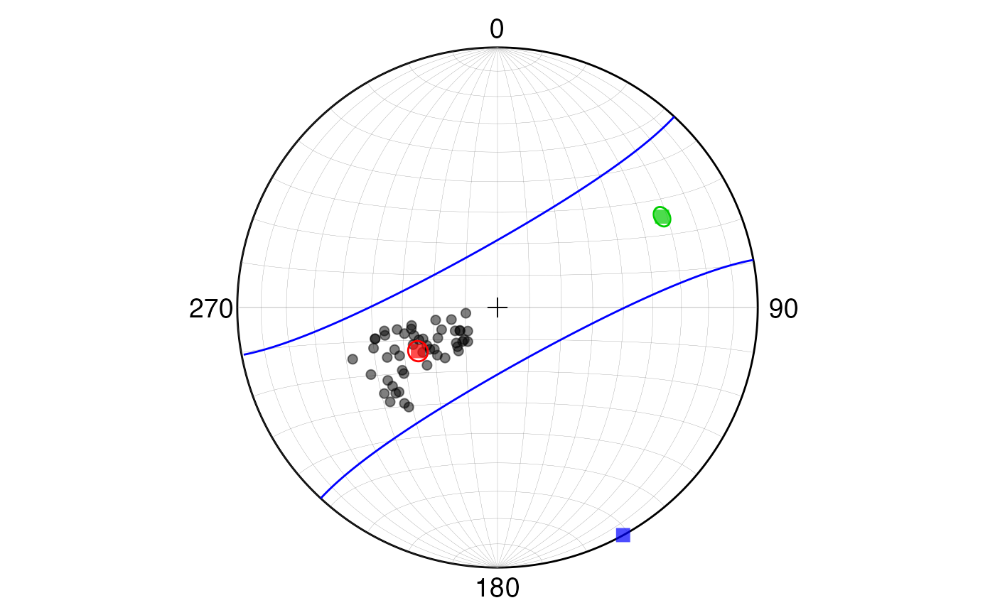# From a data frame
csv_path <- system.file("spherical_data_ax_bp.csv", package = "GMisc")
df <- utils::read.csv(csv_path)
res2 <- dir_stats_spher(dip_direction, dip, data = df,
                        conf.level = 0.90, type = "dir")
res2$axis_stats_watson
#> # A tibble: 1 × 5
#>   V1_cone V2_cone V3_cone kappa_bipolar kappa_girdle
#>     <dbl>   <dbl>   <dbl>         <dbl>        <dbl>
#> 1    2.93    2.30       0          12.6        -14.1
res2$eigenplot