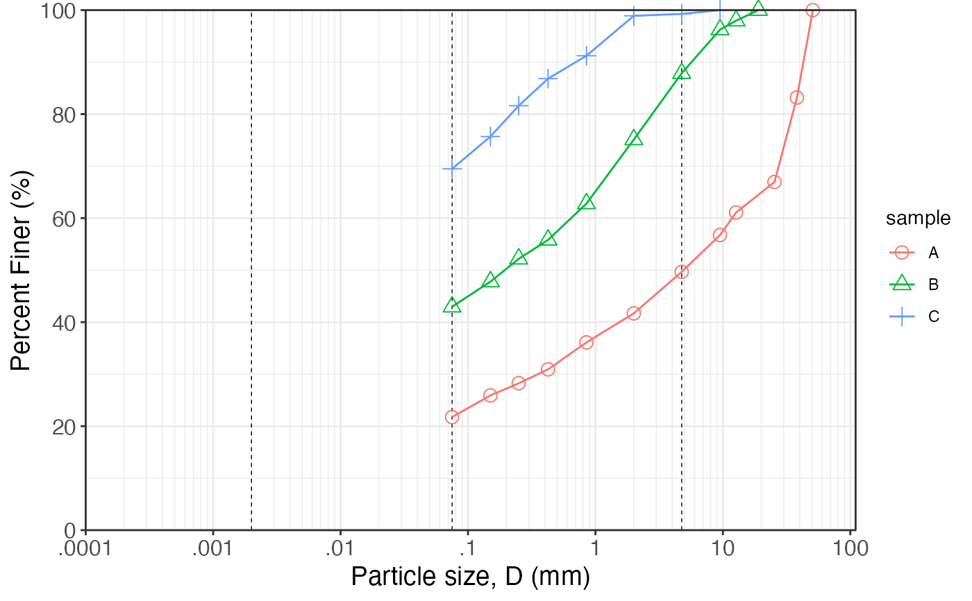
Create a template for particle size distribution graphs with logarithmic x-axis and standard vertical lines indicating common soil classification boundaries (clay/silt at 0.002 mm, silt/sand at 0.075 mm, sand/gravel at 4.75 mm). The graph is set up with appropriate axis labels and breaks for typical particle size ranges.
See also
Other soil mechanics:
Casagrande_LL(),
DS_plot(),
Mohr_Circle(),
bearing_capacity(),
compaction_test(),
fallcone_limits(),
induced_stress(),
insitu_stress()
Examples
suelo = dplyr::tribble(
 ~m      , ~m.n    , ~d     , ~pp    , ~sample  ,
 "2"     ,   2     , 50.8   , 100    , "A"      ,
 "1 1/2" ,   1.5   , 38.1   ,  83.19 , "A"      ,
 "1"     ,   1     , 25.4   ,  66.95 , "A"      ,
 "1/2"   ,    .5   , 12.7   ,  61.08 , "A"      ,
 "3/8"   ,   0.375 ,  9.5   ,  56.75 , "A"      ,
 "4"     ,   4     ,  4.75  ,  49.67 , "A"      ,
 "10"    ,  10     ,  2     ,  41.69 , "A"      ,
 "20"    ,  20     ,  0.85  ,  36.11 , "A"      ,
 "40"    ,  40     ,  0.425 ,  30.92 , "A"      ,
 "60"    ,  60     ,  0.25  ,  28.25 , "A"      ,
 "100"   , 100     ,  0.15  ,  25.91 , "A"      ,
 "200"   , 200     ,  0.075 ,  21.74 , "A"      ,
 "3/4"   ,    .75  , 19     , 100    , "B"      ,
 "1/2"   ,    .5   , 12.7   ,  97.97 , "B"      ,
 "3/8"   ,   0.375 ,  9.5   ,  96.25 , "B"      ,
 "4"     ,   4     ,  4.75  ,  87.86 , "B"      ,
 "10"    ,  10     ,  2     ,  75.11 , "B"      ,
 "20"    ,  20     ,  0.85  ,  62.8  , "B"      ,
 "40"    ,  40     ,  0.425 ,  55.82 , "B"      ,
 "60"    ,  60     ,  0.25  ,  52.18 , "B"      ,
 "100"   , 100     ,  0.15  ,  47.79 , "B"      ,
 "200"   , 200     ,  0.075 ,  42.96 , "B"      ,
 "3/8"   ,   0.375 ,  9.5   , 100    , "C"      ,
 "4"     ,   4     ,  4.75  ,  99.27 , "C"      ,
 "10"    ,  10     ,  2     ,  98.91 , "C"      ,
 "20"    ,  20     ,  0.85  ,  91.23 , "C"      ,
 "40"    ,  40     ,  0.425 ,  86.83 , "C"      ,
 "60"    ,  60     ,  0.25  ,  81.62 , "C"      ,
 "100"   , 100     ,  0.15  ,  75.70 , "C"      ,
 "200"   , 200     ,  0.075 ,  69.48 , "C"
)
particle_size_graph() +
  ggplot2::geom_point(
     ggplot2::aes(.data$d, .data$pp,
                  shape = .data$sample,
                  color = .data$sample),
     suelo, size = 3) +
  ggplot2::geom_line(ggplot2::aes(.data$d, .data$pp,
                     color = .data$sample), suelo) +
  ggplot2::scale_shape_manual(values = 1:3)