Chapman-Richards Growth Model

These functions provide Chapman-Richards equation (chaprich.fun()), as well as the self-starters for the nls() (SSchaprich()) and drc::drm() functions (DRCchaprich()).

Usage

chaprich.fun(x, a, b, c)

SSchaprich(x, a, b, c)

DRCchaprich()

Arguments

x

A numeric vector of non-negative values (e.g., time, distance).

a

The asymptote (upper limit) of the response. Must be positive.

b

The rate parameter controlling the speed of growth. Must be positive.

c

The shape parameter controlling the inflection point of the curve.

Value

chaprich.fun() and SSchaprich() return a numeric value, while DRCchaprich() returns a list containing the nonlinear function and the self starter function.

Details

The Chapman-Richards model is defined as:

$$y = a \left(1 - e^{-bx}\right)^c$$

where a is the upper asymptote, b is the rate parameter, and c is the shape parameter.

See also

Other non-linear functions, self-starters: exp3.fun(), expneg.fun(), expneg2.fun(), invpoly1.fun(), invpoly2.fun(), invpoly3.fun(), kostmod.fun(), varexp.fun(), vargauss.fun(), varsph.fun()

Examples

x <- seq(0, 10, length.out = 50)
y <- chaprich.fun(x, a = 10, b = 0.5, c = 2) + rnorm(50, sd = 0.2)
df <- data.frame(x = x, y = y)
mod = nls(y ~ SSchaprich(x, a, b, c), data = df)
summary(mod)
#> 
#> Formula: y ~ SSchaprich(x, a, b, c)
#> 
#> Parameters:
#>   Estimate Std. Error t value Pr(>|t|)    
#> a  9.93197    0.07199  137.96   <2e-16 ***
#> b  0.50011    0.01965   25.46   <2e-16 ***
#> c  1.94692    0.09700   20.07   <2e-16 ***
#> ---
#> Signif. codes:  0 ‘***’ 0.001 ‘**’ 0.01 ‘*’ 0.05 ‘.’ 0.1 ‘ ’ 1
#> 
#> Residual standard error: 0.1951 on 47 degrees of freedom
#> 
#> Number of iterations to convergence: 6 
#> Achieved convergence tolerance: 6.176e-07
#> 
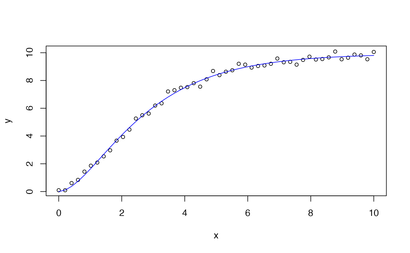
plot(x,y,cex=.8)
lines(x,predict(mod),col='blue')


if (FALSE) { # \dontrun{
mod = drc::drm(y ~ x, data = df, fct = DRCchaprich())
summary(mod)
plot(mod, log = "")
} # }