These functions provide Two-Asymptote Exponential Model equation (expneg2.fun()), as well as the self-starters for the nls() (SSexpneg2()) and drc::drm() functions (DRCexpneg2()).
Arguments
- x
A numeric vector of values (e.g., time, dose).
- a
The initial asymptote: the value of the response as
xapproaches zero (or negative infinity).- b
The final asymptote: the value of the response as
xtends to infinity.- c
The rate parameter in the exponent. Negative values yield a transition from
atowardbasxincreases.
Value
expneg2.fun() and SSexpneg2() return a numeric value, while DRCexpneg2() returns a list containing the nonlinear function and the self starter function.
Details
The model is defined as:
$$y = a \, e^{cx} + b \left(1 - e^{cx}\right)$$
This can be rearranged as \(y = b + (a - b)\,e^{cx}\), making clear that
the curve transitions from a at \(x = 0\) to b as
\(x \to \infty\) (when \(c < 0\)). a is the initial asymptote,
b is the final asymptote, and c is the rate parameter.
See also
Other non-linear functions, self-starters:
chaprich.fun(),
exp3.fun(),
expneg.fun(),
invpoly1.fun(),
invpoly2.fun(),
invpoly3.fun(),
kostmod.fun(),
varexp.fun(),
vargauss.fun(),
varsph.fun()
Examples
x <- seq(0, 10, length.out = 50)
y <- expneg2.fun(x, a = 2, b = 8, c = -0.4) + rnorm(50, sd = 0.2)
df <- data.frame(x = x, y = y)
mod = nls(y ~ SSexpneg2(x, a, b, c), data = df)
summary(mod)
#>
#> Formula: y ~ SSexpneg2(x, a, b, c)
#>
#> Parameters:
#> Estimate Std. Error t value Pr(>|t|)
#> a 2.03122 0.11466 17.71 <2e-16 ***
#> b 7.99592 0.06815 117.33 <2e-16 ***
#> c -0.40407 0.01873 -21.58 <2e-16 ***
#> ---
#> Signif. codes: 0 ‘***’ 0.001 ‘**’ 0.01 ‘*’ 0.05 ‘.’ 0.1 ‘ ’ 1
#>
#> Residual standard error: 0.1993 on 47 degrees of freedom
#>
#> Number of iterations to convergence: 3
#> Achieved convergence tolerance: 4.027e-07
#>
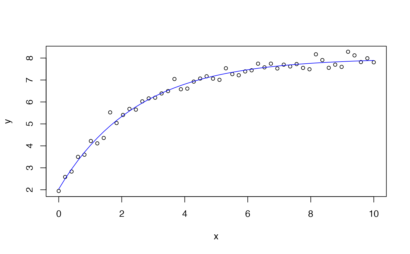
plot(x, y, cex = 0.8)
lines(x, predict(mod), col = 'blue')
 if (FALSE) { # \dontrun{
mod = drc::drm(y ~ x, data = df, fct = DRCexpneg2())
summary(mod)
plot(mod, log = "")
} # }
if (FALSE) { # \dontrun{
mod = drc::drm(y ~ x, data = df, fct = DRCexpneg2())
summary(mod)
plot(mod, log = "")
} # }