These functions provide Spherical Variogram Model equation (varsph.fun()), as well as the self-starters for the nls() (SSvarsph()) and drc::drm() functions (DRCvarsph()).
Arguments
- x
A numeric vector of non-negative lag distances.
- nug
The nugget: the semivariance at zero lag distance (intercept).
- psill
The partial sill: the difference between the sill (total variance) and the nugget.
- range
The range parameter: the lag distance at which the sill is reached and spatial autocorrelation ceases. Beyond this distance the semivariance is constant at
nug + psill.
Value
varsph.fun() and SSvarsph() return a numeric value, while DRCvarsph() returns a list containing the nonlinear function and the self starter function.
Details
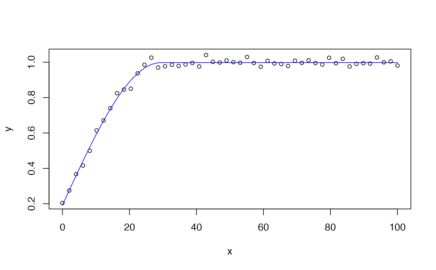
The model is defined as:
$$y = \begin{cases} \text{nug} + \text{psill} \left(\frac{3}{2}\frac{x}{\text{range}} - \frac{1}{2}\left(\frac{x}{\text{range}}\right)^3\right) & x \leq \text{range} \\ \text{nug} + \text{psill} & x > \text{range} \end{cases}$$
where nug is the nugget, psill is the partial sill, and
range is the lag distance at which the sill is reached exactly.
Unlike exponential and Gaussian models, the spherical model reaches the
sill at a finite distance.
Unlike the exponential and Gaussian models, the spherical model reaches the
sill exactly at a finite distance (range), making it suitable when a hard
limit on spatial dependence is expected.
See also
Other non-linear functions, self-starters:
chaprich.fun(),
exp3.fun(),
expneg.fun(),
expneg2.fun(),
invpoly1.fun(),
invpoly2.fun(),
invpoly3.fun(),
kostmod.fun(),
varexp.fun(),
vargauss.fun()
Examples
x <- seq(0, 100, length.out = 50)
y <- varsph.fun(x, nug = 0.2, psill = 0.8, range = 30) + rnorm(50, sd = 0.02)
df <- data.frame(x = x, y = y)
mod = nls(y ~ SSvarsph(x, nug, psill, range), data = df)
summary(mod)
#>
#> Formula: y ~ SSvarsph(x, nug, psill, range)
#>
#> Parameters:
#> Estimate Std. Error t value Pr(>|t|)
#> nug 0.19198 0.01126 17.05 <2e-16 ***
#> psill 0.80581 0.01152 69.97 <2e-16 ***
#> range 29.27413 0.54626 53.59 <2e-16 ***
#> ---
#> Signif. codes: 0 ‘***’ 0.001 ‘**’ 0.01 ‘*’ 0.05 ‘.’ 0.1 ‘ ’ 1
#>
#> Residual standard error: 0.01864 on 47 degrees of freedom
#>
#> Number of iterations to convergence: 3
#> Achieved convergence tolerance: 1.592e-07
#>
plot(x, y, cex = 0.8)
lines(x, predict(mod), col = 'blue')
 if (FALSE) { # \dontrun{
mod = drc::drm(y ~ x, data = df, fct = DRCvarsph())
summary(mod)
plot(mod, log = "")
} # }
if (FALSE) { # \dontrun{
mod = drc::drm(y ~ x, data = df, fct = DRCvarsph())
summary(mod)
plot(mod, log = "")
} # }